Summary PivotTables are used to summarize, analyze, explore and present data. PivotCharts complements PivotTables by adding visualizations to the summary data in a PivotTable and allows you to easily visualize comparisons, patterns, and trends. PivotTables and PivotCharts both enable you to make informed decisions about the important data in your enterprise. You can also connect to external data sources such as SQL Server Tables, SQL Server Analysis Services Cubes, Azure Marketplace, Office Data Connection (.odc) files, XML files, Access databases, and text files to create PivotTables or use existing PivotTables Huh. Create new tables.
ComputerSolve Explains PivotTables
Pivot table in excel is used to classify, sort, filter, and summarize any length of data table which we can get count, sum, value in form of table or as 2 column set. To insert a pivot table, choose the Pivot Table option from the Insert menu tab, which will automatically find the table or range. We can also use the shortcut keys Alt + D + P together, which will let us explore the range of cells and take us to the last pivot option. We can also create a customized table by actually considering the required columns.
PivotTable is an interactive way to quickly summarize large amounts of data. You can use a Pivot Table to analyze numerical data in detail and answer unexpected questions about your data. PivotTable is specifically designed to :
- Querying large amounts of data in multiple user-friendly ways.
- Subtract and collect numerical data, summarize data by categories and subcategories, and create custom calculations and formulas.
- Expand and collapse the level of data to focus your results on, and drill down from summary data to the description for your areas of interest.
- Moving (or “pivoting”) rows into columns or rows into columns to see different summaries of the source data.
- Filtering, sorting, grouping, and conditional formatting enable you to focus only on the information you want, which is the most useful and interesting subset of data.
- Submit a concise, attractive, and annotated report online or in print.
How to get an excel power pivot add-in?
Power Pivot gives you the power of a business insight and analytics app. You don’t need special training to develop and calculate data models. You just need to enable it before using it.
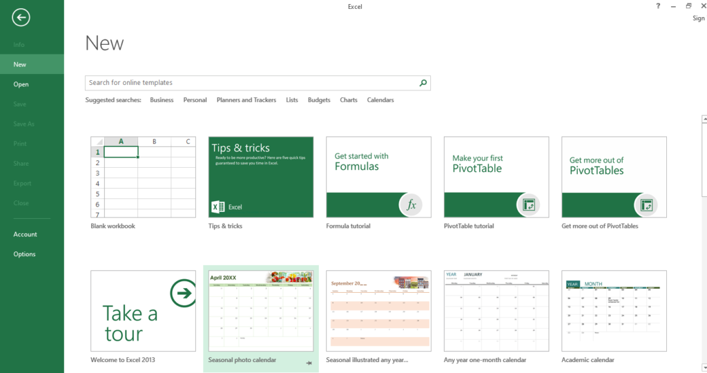
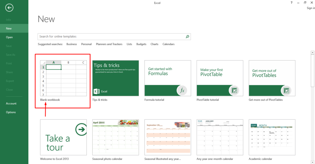
- Open Excel.
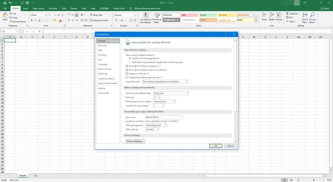
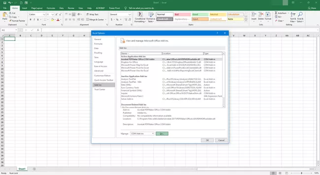
2. Select File > Options.
3. Select Add-ins.
4. Select the Manage dropdown menu, then choose COM Add-ins.
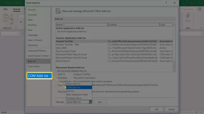
5. Select Go.
6. Select Microsoft Power Pivot for Excel.
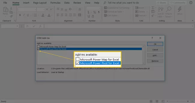
7. Select OK. The Power Pivot tab is added to Excel.
Related: how to delete a pivot table
How to Create a Pivot Table in Excel?
To create a pivot table in Excel, you need to perform the following steps :
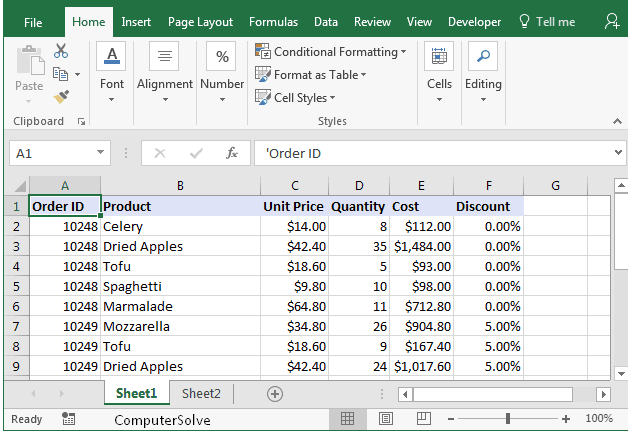
- Before we begin, we would like to first show you the data for the pivot table. In this example, the data is found on Sheet1.
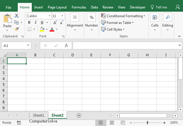
- Highlight the cell where you want to create the pivot table. In this example, we have selected cell A1 on Sheet2.
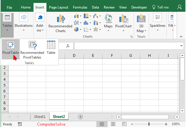
- Next, select the Insert tab from the toolbar at the top of the screen. In the Tables group, click the Tables button and choose PivotTable from the popup menu.
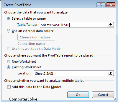
- The Create a Pivot Table window should appear. Select the range of data for the pivot table and click the OK button. In this example, we selected cells A1 through F16 in Sheet1 as indicated by Sheet1!$A$1:$F$16.
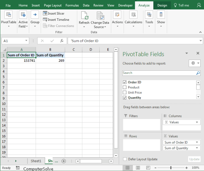
Your pivot table will now look like this :
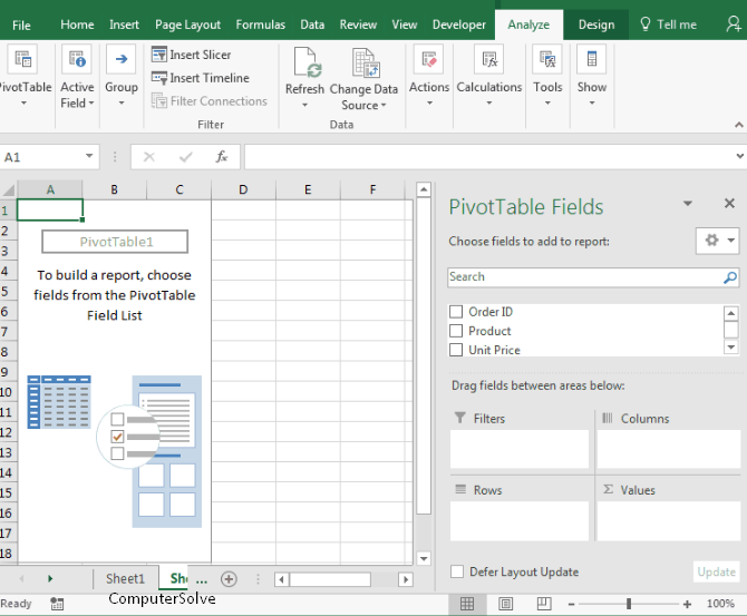
- Next, select the field to add to the report. In this example, we selected the checkboxes next to the Order ID and Quantity fields.
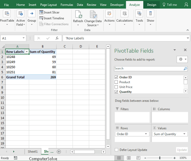
- Then, Next in the Value section, click on “Sum of Order ID” and drag it to the Row section.
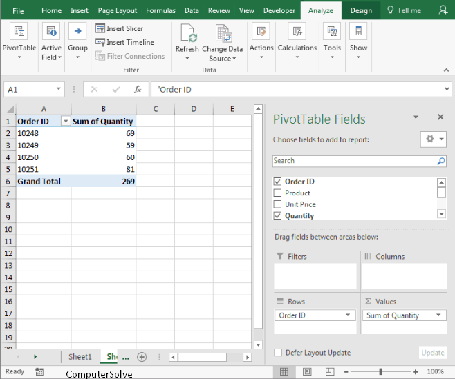
- Lastly, we want the title in cell A1 to appear as “Order ID” instead of “Row Label“. To do this, select cell A1 and type the order ID.
Your pivot table should now display the total quantity for each order ID as follows :
Congratulations, you have created your first pivot table in Excel