
Excel sheets are the best program that is designed by Microsoft for data analysis. It also helps with documentation and has some excellent features, such as graphing tools, computation capabilities, pivot tables, and it also has a macro programming language.
The visual appearance of the Microsoft sheets consists of columns and rows which is best for data tabulation. It is being used in schools, colleges, and mostly in offices to manage the work and keep a record.
If your project involves data analysis and you need to perform basic arithmetic calculations, such as multiplication, addition, subtraction, and division, then this guide is for you.
Today, we are going to share the pro tips on how to subtract in excel. And, we will also discuss the formula for numbers, percentages, dates, and times. Here you will learn to subtract across cells, columns, rows and varied ranges.
Let’s begin with the basics and after that, we will also discuss the complex arithmetic and advanced process to solve it.
Must Read – How to Subtract in Google Sheets?
Subtracting Cells/Values in Microsoft Excel

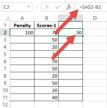
We will take the help of two numbers say 20 and 10 to provide you get a clear idea about the process. Now, if you want to subtract 20 and 10, then you need to input these values in one of the cells first. Then, select a cell where you want the result to appear, there you need to enter the “=” sign.
Now, put the first value that you have to subtract from, right next to the sign. Place a subtraction sign “-” and put the second number that you want to subtract. The fx or formula bar would look something like this fx “=20-10”. Now, hit the Enter key and you would be able to view the result in the selected cell. This syntax is also called the formula in Excel because an equal-to sign is used to get the desired result.
This was a manual method, and you have to put the numbers manually. You can use the same formula to resolve all the other number sets that are meant to be subtracted in this Microsoft Excel.
Now, if you do not want to enter the number manually, then you can put the cell number. For example, if you have placed the numbers 20 and 10 in the cells A4 and A5 respectively, then your fx or formula bar would look like “=A4-A5”. (Remember, there is no space in between the signs of numbers).
Similarly, you can use the cell reference to get the values for the rest of the set. Thus, you do not need to change the values every time, the formula would get updated automatically and would show you the results.
This involves an advanced way of subtracting more than two values. Suppose, you have an entire column filled with values and you have to conduct a subtraction between these two sets of columns, then worry not, Excel serves to be the best medium for that.
Let’s say you have an entire column starting from A4 to A12 filled with numbers and from each of them, you have subtracted a value say 5. Then, right next to A4 is B4, select it and in the fx bar enter the formula “=B4-5”. Now, copy cell B4, select the entire column from B5 to B12 and paste the copied cell. You will notice that the formula has been modified according to the cell number and applied to the selected column.
This happens because you have used B4 as the cell reference. You can also use a shortcut, i.e. select the result cell B4 and drag it would let go of the mouse. This would impart a similar result and would also reduce your time.
Irrespective of the Microsoft version you are using, every Excel works in a similar pattern. But, if you are using Microsoft 365, then you gain an upper hand, the formula becomes a bit easier. But, before you start you need to put the number to be subtracted in a cell, say D2.
Here instead of fx “=B4-5” you can enter “B4:B12-D2”, depicting the entire column. Now, hit the Enter key and you will get the desired result. This shortcut works on an array of values and so it is called the dynamic array formula.
Subtract Percentage in Excel
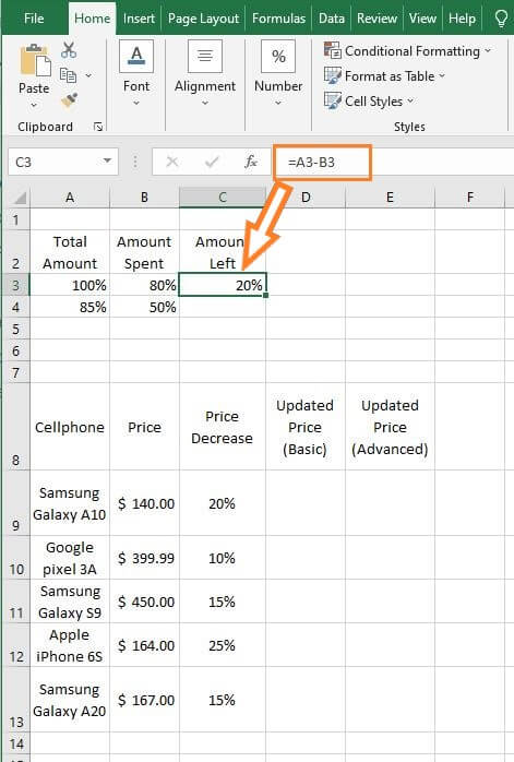
What if we told you that you can subtract percentages in Excel. The formula is quite simple, say you want to subtract 50% from 80%, then you have to place the formula as fx “=80%-50%”. Otherwise, you can also put the individual cell number and select the result cell (where you want the number to appear), say fx “=D4-D6”.
Now, if you want to subtract a percentage from a number, then you need to use this formula fx “=Number*(1-#%)” (Here # represents the percentage value). So, if you want to know how can you reduce the number in D4 by 20%, then it would appear as “=D4*(1-20%)”.
If you want to calculate the value for a column, then you need to put the percentage in a separate cell say G4, and then put the formula as fx “=D4*(1-$G$4)”.
Subtract Dates in Excel
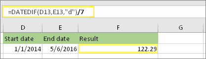
The most interesting feature of Microsoft Excel is that all the Dates and Time values are stored in the backend. For example, the date 01 Jan 2021 is represented by 44197. This feature helps to subtract the dates easily without much hassle.
Suppose, you have two dates, then using Excel you can calculate the number of days elapsed between the dates. Now, let’s create 3 columns, the first one would consist of the starting date, the second one would consist of the end date and the last column would have the difference of days elapsed.
Now, if you have placed the starting date in D3 and the ending date in E3, then the formula would be fx “=E3-D3”. Select the F3 enter the formula and hit the Enter button, you will get the number of days elapsed.
Often Excel tries to be helpful and provide the result in the exact format that you have placed in the adjacent column. You have the option to choose the format. Go to the Home tab and from the drop-down list select General in the number. But, remember, Excel would work in this format only if it recognizes the values, otherwise, it would treat the dates as text strings.
Subtract Time in Excel
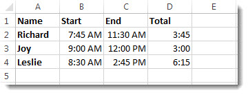
Subtracting time in Excel also follows a similar pattern. You need to use the formula fx “=end_time-start_time”. Suppose, you have listed the end time in C2 and start time in B2. Then, you need to use this formula fx “=C2-B2”. Select a cell where you would want the result to be displayed, and then place the syntax in the formula bar.
Now, if you want the result to be displayed in the Time format, then you need to maintain the format in the Start time and End time list. Otherwise, Excel would fail to recognize the string.
If you want to save time, then you can use the TIME VALUE function directly, say TIMEVALUE(“5:30PM”)-TIMEVALUE(“1:00PM).
Read – Name Box In Excel
Conclusion
So, now, you are accustomed to how to subtract numbers, percentages, dates as well as times in Excel. Similarly, you can also do matrix subtraction, subtract one list from another, and many more. Keep following our blogs to get a quick hack and complete guide to work on Excel.