When you are subtracting or performing any arithmetic expression on paper, then you use symbols, and these are either “-” or “+” or “/” or “*”, etc. Google Sheets work somewhat in a similar pattern. But, there is the only difference you will get and that is the usage of cells instead of relying solely on numbers.
In Google Sheets, you will get a specific box to write the formula, and this is also known as the formula bar. And, the advantage is that with just a single formula you can solve 100 and more subtraction arithmetic. Here you will notice separate colours are being used for designation, and each of these colours in the formula represents the cell that you have chosen. The colours basically help you to keep track and based on that you can also elongate the formula or add more parts to it.
But, always remember to double-check the syntax of the formula that you are about to use. Further, you also get the benefit of mixing cell numbers as well as values to obtain the exact result, for example, you can write “=120-A6-B8”. You can also choose any number and any cell number.
Here, in this guide, we are about to discuss the most used and common ways of subtracting numbers in Google Sheets. It is quite similar to Microsoft Excel and you don’t need to have the technical know-how to proceed.
Also Rrad -Arrow keys not working in excel
Terms to Remember
Before we proceed with the subtractions, here are a few terms that you must remember. While calculating, the fact that what should be calculated at first is called the order of operation. Next comes the word Parenthesis, which is the order that forms the innermost to the outermost parens. You will also get the word Exponents, it is used to denote the caret symbols. Other than this, you are quite familiar with the terms, multiplication, division, addition, and subtraction, and these are rendered with these symbols: *, /, +, and – respectively.
Now that you have acquired the basic idea, let’s proceed to the steps that you need to implement to subtract a set of numbers in a Google Sheet.
Use the MINUS function
This is the most simple and basic step that you would love to learn. Microsoft Excel and Google Sheets have distinct functions for arithmetic functions. In the Google Sheets, you get the MINUS function and it is workable through numbers and cell references as well. When you are working with two arguments, then the syntax for the formula is MINUS(value1, value2).
For example,
There are two arguments 10 and 5 and you have to subtract the numbers.
You need to enter the designated formula and finally hit the Enter button.
Here’s how it is going to get depicted as “=MINUS(10,5)”. The end process will provide the result.
Now, suppose you need to subtract the values within cells, then need to put the cell number and it can be
A2, A3 or B4, B6, etc. So, you have to put that right after the fx term of the formula bar “=MINUS(A3, A4)”. Here, you can change the value/numbering of the cell based on the preference. You can subtract either horizontally or vertically.
Use the Minus Sign
Instead of using the MINUS function you can also try and use the minus sign and it would work the same way. Based on the cells or numbers that you prefer, you can go for the “-” symbol.
Here is an advantage, you do not have to include the values in parentheses, for example – to subtract numbers, such as 10 minus 5, you have to enter “=10-5” and then hit the Enter button. This will provide you with the result.
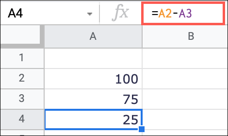
Similarly, you can also put the cell numberings, such as A2 or A3, or B5 or B6, then enter the formula and press the Enter key.
For example “B5-B6”. These formulas are useful only when you are working with two numbers that you want to subtract. However, the list can go on for more than 100 such grouped numbers.
Use the SUM function
Now, you must be wondering how is this even possible that by using the SUM function you can subtract any values. But, let us tell you that it is possible. If you know how to use the SUM function, then we would suggest that you keep using it. So, let’s see how the SUM function can help you to subtract.
Here is the formula that you would be using “=SUM(10-5)” or if you are using the cell numberings, then it would be “=SUM(A3-A4)”. You can change the cell numbers based on your preferences.
But, always remember that after entering the formula you need to press the Enter key to get the desired results.
Create Subtraction Equation
Now, every calculation might not be as simple as it appears, as in A minus B. You might even need to deal with complex problems. Suppose, you might need to add a few numbers and then subtract a few. Thus, you need to solve such complex problems using the functions as well as the operators, such as the plus signs and the minus signs. You can create the equation based on the demand of the problem.
Related Post-
How to fix excel ran out of resources
And, Here is how you can proceed:
If you need to use the MINUS function to subtract any values, then you can multiply them as well. You can use this formula =MINUS(A3,A4)*10. Here you need to subtract the values that would be put in the cells A3 and A4, and then you would be multiplying the results by 10 end values. But, after you have put the formula next to the fx box, i.e. the formula bar, hit the Enter key. Otherwise, you would not get the end result.
In exactly the same way you can also add the values after subtracting them based on your cell preferences. Using somewhat a similar formula you can subtract 5 from 15 and then add 5 more to the result. Here you get the advantage to use the parentheses with the minus sign, and then you get to go through the calculation. For example, here is the formula that you have to type in next to the fx box or formula bar “=(15-5)+5”.
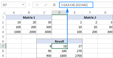
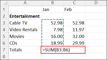
What if you have to add a range of numbers, and then you need to subtract it from another number. In this case, you have to use the SUM function, and then add the range of values in the cells (say from A4 to A9), and after this subtract it with a number placed in the cell, say A10. The formula would appear as “=SUM(A4:A9)-A10”
What About Complex Arithmetic Problems?
In a similar way, you can also divide the number either after subtracting or dividing and then subtract the result with another number. These are basic calculations and you can follow the exact pattern to create something that would provide you with the desired result.
Conclusion
Actually, there is no limit to the number of terms, values, or functions that can be used to create a formula. If the formula is syntactically correct, then you can easily proceed. Even if the formula is “=((4+4)^4)*(SUM(A2:A8)-150*(MINUS(C5,D31)”. You can use these formulas for solving complex problems in your final statement report or for the year-end reports.