Excel is very easy and convenient way for sorting large amount of data, since it involves different kind of editing and formatting. When you want to organize the data, you may find it helpful to unhide excel columns as per your convenience. You can hide, and then unhide whenever you want, columns by right clicking in the spreadsheet or you can also achieve this with the help of a drop-down menu in the home tab.
What are the solutions of unhide columns in excel ?
It is essential to know the way to unhide data. Here we’ll notify and discuss briefly about seven different methods to unhide excel columns we’ll discuss :
- Home tab of Excel Ribbon
- Shortcut Key
- Context Menu
- Column Width
- Ctrl+G (go to) Command
- Ctrl+F (find) Command
- Double-line Icon
Method 1 – Home Tab of Excel Ribbon
- First of all, select the columns to the left and right of the hidden column.
- Next, In the Home tab, under the ‘cells‘ group, click the ‘format‘ drop-down option.
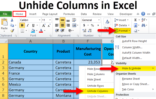
- As you’ll see, from the ‘hide and unhide’ option, you need to select ‘unhide columns’ to complete the process.
Method 2 – Shortcut Keys
- Firstly, select the columns to the left and right of the hidden column.
- After that, Press the shortcut ‘Alt H O U L’, Press one key at a time.
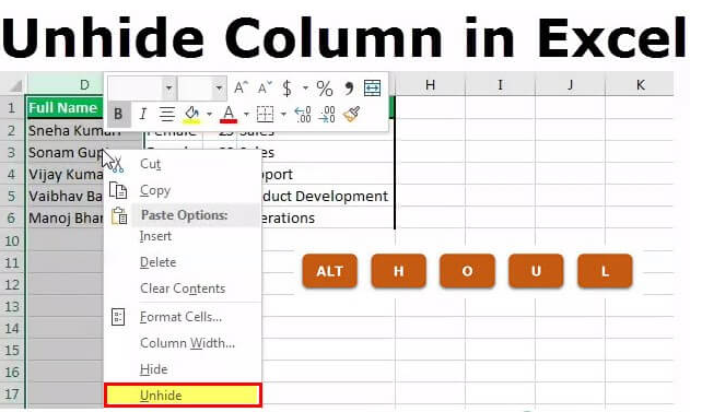
Method 3 – Context Menu
- Initially, select the columns to the left and right of the hidden column.
- Then right-click on the selected columns and choose ‘unhide‘ option.
Method 4 – Column Width
- First select the columns to the left and right of the hidden column.
- Now, right click on the selected columns and then choose ‘column width’.
- After this step, enter any number as the ‘column width’.
Method 5 – Ctrl+G (Go To) Command
In a succeeding image, column ‘B and C’ are hidden.
- Then, in the Home tab, click ‘find and select’ drop-down and choose ‘go to’.After that, you need to press the shortcut key ‘F5’.
- In the next step, Specify any cell reference of the hidden column just like ‘B1:C1’ in the ‘go to’ dialog box. Then click ‘Ok’.
- Now, as per your choice, choose any preceding methods as we discussed earlier to unhide columns ‘B and C’.
Method 6 – Ctrl+F (Find) Command
In the succeeding image, column B and C are hidden.
- First of all, you need to press ‘Ctrl+F’ and then as you’ll see the ‘find and replace’ dialog box appears.
- After that, enter the data of one of the hidden cells in the ‘find what’ box.
- Then click ‘options>>’ and select the given check box ‘match entire cell contents’.
- Now, click ‘find next’ and close the ‘find and replace’ dialog box.
- Select any preceding methods as given above to unhide columns ‘B and C’.
Method 7 – Double Line Icon
- At the initial step, enter a single cell reference of the hidden column in the ‘Name’ box. This box is placed to the left side of the formula bar.
- Then press the ‘Enter’ key.
- Now, you should select the columns to the left and right of the hidden column.
- Then double-click ‘the double-line icon'(having arrows pointing to the left and right) in-between the column labels.
- At the final step, follow one of the methods that we discussed above, to unhide the column.