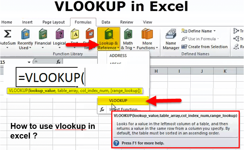
The VLOOKUP function in Excel is used to find something in a table. If you have rows of data arranged by column headings, VLOOKUP can be used to find the value using a column.
When you perform a VLOOKUP, you are telling Excel to first locate the row that contains the data you want to retrieve, and then to return the value located in a specific column within that row.
The VLOOKUP function uses the following arguments :
- Lookup value (argument required) – Lookup_value specifies the value we want to look for in the first column of the table.
- Table array (arguments required) – The table array is the data array that is to be searched. The VLOOKUP function searches the leftmost column of this array.
- Col index num (required argument) – This is an integer, specifying the column number of the supplied table_array from which you wish to return a value.
- Range lookup (optional argument) – defines what this function will return if it does not find an exact match to the lookup value. The argument can be set to TRUE or FALSE, which means :
- TRUE – Predicted match, that is, if no exact match is found, use the closest match below the lookup_value.
- FALSE – Exact match, i.e. if no exact match was found, it will return an error.
VLOOKUP Function Example –
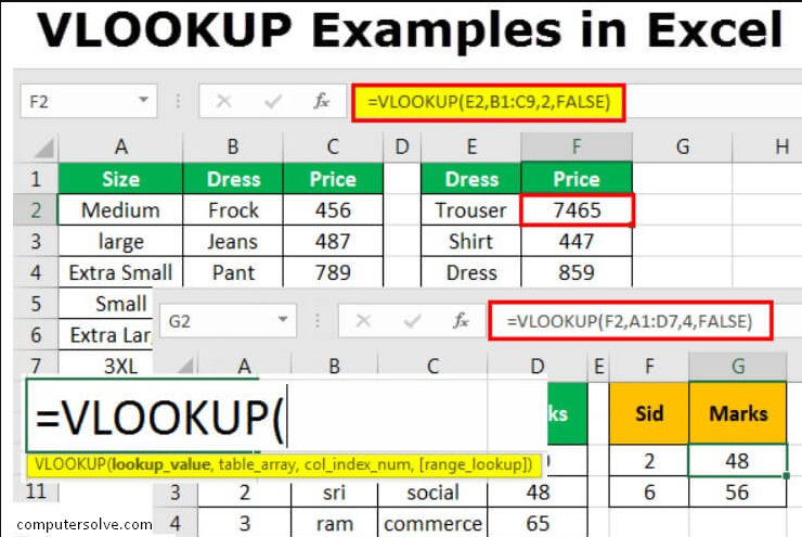
Here are some examples showing the VLOOKUP function in action :
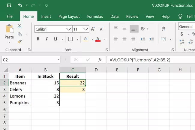
=VLOOKUP("Lemons",A2:B5,2)
This is a simple example of the VLOOKUP function where we need to find out how many lemons we have from a list of multiple items. The range we are looking at is A2:B5 and the number we need to pull is in column 2 because “in stock” is the second column from our range. Here the result is 22.
See: how to lock a cell in excel
Find an Employee’s Number Using Their Name –
=VLOOKUP(A8,B2:D7,3)
=VLOOKUP(A9,A2:D7,2)
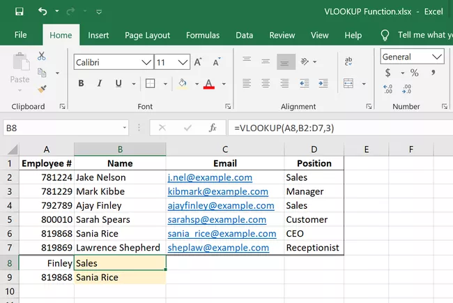
Here are two examples where we write the VLOOKUP function a little differently. They’re both using the same data set, but since we’re pulling information from two different columns, 3 and 2, we make up that difference at the end of the formula the first one being the person in A8 (Finale). is the situation. , Whereas the second formula returns the name that matches the employee number in A9 (819868). Since formulas are reference cells and not specific text strings, we can omit the quotes.
VLOOKUP ERRORS AND RULES
Here are a few things to remember when using the VLOOKUP function in Excel :
- If search_value is a text string, it must be surrounded by quotes.
- If VLOOKUP does not find any result, Excel will return #NO MATCH.
- If there is no number in the lookup_table that is greater than or equal to search_value, Excel will return #NO MATCH.
- Excel will return #REF! If the column_number is greater than the number of columns in the lookup_table.
- The search_value is always at the far left of the lookup_table and the position is 1 when determining the column_number.
- If you specify FALSE for predicted_match and no exact match is found, VLOOKUP will return #N/A.
- If you specify TRUE for predicted_match and no exact match is found, the next smaller value is returned.
- Unsorted tables must use FALSE for predicted_match so that the first exact match is returned.
- If predicted_match is true or omitted, the first column needs to be sorted either alphabetically or numerically. If it is not sorted, Excel may return an unexpected value.
- By using absolute cell references you can auto-populate formulas without changing the lookup_table.
See: how to create a drop down list in excel