
Drop-down lists are helpful in Excel. Create a drop-down list in Excel and you can help people work more efficiently in worksheets by using drop-down lists in Excel. The drop-down allows people to select an item from a list you’ve created.
In this article, we will show you how you can create a drop-down list in Excel. It also provides information on using the list for data validation options, protecting the drop-down list, and making changes to the drop-down list.
What is data validation?
Data validation is a tool that helps you control the information you enter on your worksheets. With Data Validation, you can :
- Provide users with a list of options.
- Restrict entries to a specific type or size.
- Create custom settings.
In this tutorial, you will see how to create a drop-down list of options in a cell.
Related: how to lock a cell in excel
How to enter data to create a drop-down list?
When you add a drop-down list to a cell in Excel, an arrow appears next to it. Clicking on the arrow opens the list so you can select one of the items to enter into the cell. For example, if you’re using a spreadsheet to track RSVPs for an event, you could filter that column by Yes, No, and Not Yet Replied.
The data used in the list can be located on the same sheet as the list, on a different sheet in the same workbook, or in a different workbook. In this example, the drop-down uses a list of entries located in a different workbook. The advantages of this method include centralizing list data for multiple users and protecting it from accidental or intentional change.
- Open two blank Excel workbooks.
- Save one workbook with the name data-source.xlsx. This workbook will contain the data for the drop-down list.
- Save the second workbook with the name drop-down-list.xlsx. This workbook will contain the drop-down list.
- Leave both workbooks open after saving.
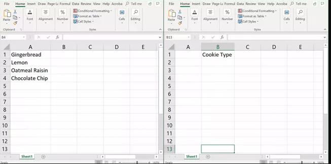
- Enter the data as shown below into cells A1 to A4 of the data-source.xlsx workbook as seen in this image.
- Save the workbook and leave it open.
- Enter the data as shown in the image into cell B1 of the drop-down-list.xlsx workbook.
- Save the workbook and leave it open.
Related: name box in excel
Data for Cells A1 to A4 in data-source.xlsx
- A1 — Gingerbread
- A2 — Lemon
- A3 — Oatmeal Raisin
- A4 — Chocolate Chip
Data for Cell B1 in drop-down-list.xlsx
- B1 — Cookie Type
How to create a drop-down list in excel?
Excel drop-down list has a useful feature that enables us to select a value from the list box. A drop-down list in excel is mainly used for data entry and organization such as medical transcription and validation data in the data dashboard to select and update in an easy way from the drop-down list. So the excel drop-down list saves time where we can avoid errors in the validation part.
We can easily create a drop-down list in excel by choosing the data tab where we can find the data validation option.
The First Named Graded :
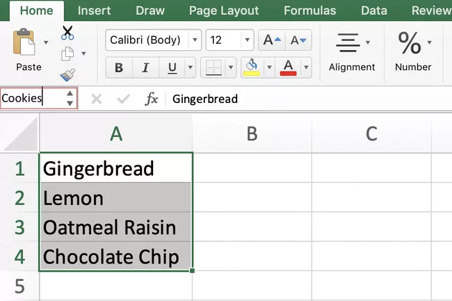
- Select cells A1 to A4 of the data-source.xlsx workbook to highlight them.
- Click on the Name Box located above column A.
- Type Cookies in the Name Box.
- Press the Enter key on the keyboard.
- Cells A1 to A4 of the data-source.xlsx workbook now have the range name of Cookies.
- Save the workbook.
The Second Named Graded :
The second named range does not use cell references from the drop-down-list.xlsx workbook. Instead, it links to the Cookies range name in the data-source.xlsx workbook, which is necessary because Excel will not accept cell references from a different workbook for a named range. It will, however, accept another range of names.
Creating the second named range, therefore, is not done using the Name Box but by using the Define Name option located on the Formulas tab of the ribbon.
Related: how to unhide excel workbook
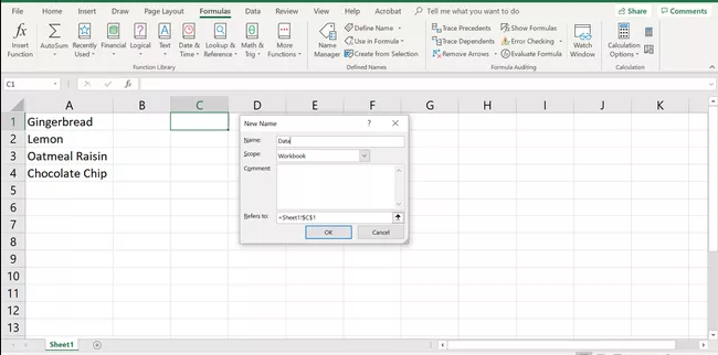
- Click on cell C1 in the drop-down-list.xlsx workbook.
- Click on Formulas > Define Name on the ribbon to open the Define Name dialog box.
- Click on the New button to open the New Name dialog box.
- Type Data in the Name line.
- In the Refers to line type =’data-source.xlsx’!Cookies
- Click OK to complete the named range and return to the Define Name dialog box.
- Click Close to close the Define Name dialog box.
- Save the workbook.
How to use the list for data validation?
All data validation options in Excel, including drop-down lists, are set using the Data Validation dialog box. In addition to adding drop-down lists to a worksheet, data validation in Excel can also be used to control or limit the type of data that users can enter into specific cells in the worksheet.
- Firstly, Click cell C1 of the drop-down-list.xlsx workbook to make it the active cell – this is where the drop-down list will be.
- Then, Click the Data tab of the ribbon menu above the worksheet.
- Then, Click the Data Validation icon on the ribbon to open a drop-down menu. Select the Data Validation option.
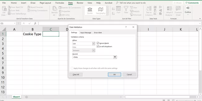
- Click the Settings tab in the Data Validation dialog box.
- Then, Click the down arrow at the end of the Allow line to open the drop-down menu.
- Then, Click the List to select drop-down list for data validation in cell C1 and activate the Source line in the dialog box.
- Because the drop-down list’s data source is in a different workbook, the second named range moves to the Source row in the dialog box.
- Then, Click on the Source line.
- In the source line type = data.
- Then, Click OK to complete the drop-down list and close the Data Validation dialog box.
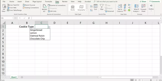
- A small down arrow icon should appear on the right side of cell C1. Clicking the down arrow will open a drop-down list containing the four cookie names entered in cells A1 to A4 of the data-source.xlsx workbook.
- Then, Click a name in the drop-down list and enter that name in cell C1.
How to change the drop-down list?
Since this example used a named range as the source for our list items instead of the actual list names, changing the cookie names in the named range in cells A1 to A4 of the data source. The xlsx workbook is immediately renamed in the drop-down list.
Follow the steps below to convert lemon to shortbread in the drop-down list by changing the data in cell A2 of the named range in the data-source.xlsx workbook.
- Firstly, Click cell A2 in the data-source.xlsx workbook to make it the active cell.
- Then, Type shortbread in cell A2 and press the Enter key on the keyboard.
- Then, In cell C1 of the drop-down-list.xlsx workbook, click the down arrow for the drop-down list.
- Item 2 on the list should now read Shortbread instead of Lemon.