How to Alphabetize a Column in Excel?

This guide will show you how to sort Excel alphabetically using sorting and filtering functions to organize your data from A to Z. This feature is especially useful for large datasets whose manual processing – alphabetical information in Excel takes a long time.

Things to know

Alphabetizing of a column or list means arranging the list alphabetically in Excel. This can be done in two ways, in descending order or in descending order.

Uses of Alphabetic sorting in Excel

It makes the data more sensible.
It gives you the ease to search values based on alphabetical order.
It also makes it easier for you to visually identify duplicate records in your data set.

Method 1 – Alphabetize using options from Excel Ribbon

This is one of the easiest ways to organize data in Excel. To use this method, follow these steps:

First select the list you want to sort.

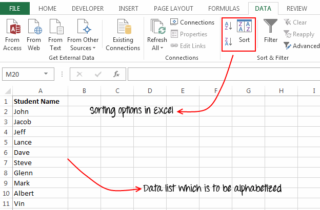
Next, navigate to the “Data” Tab on the Excel ribbon and click the “A-Z” icon for ascending order sort or the “Z-A” icon for descending sort.

Sort a multi-column data table using this method:

If there is a list with two columns, such as “Student Name” and “Role Number”. And you have to make this list based on “Student Name”. Then you should use the “Sequence” button instead of the “A-Z” and “Z-A” buttons.

The sort button gives you more control over how you want to sort the list. It allows you to select only one sequence of columns, takes care of the headers of your table, and can calculate data based on font or text color.

Follow the below steps to use this method:

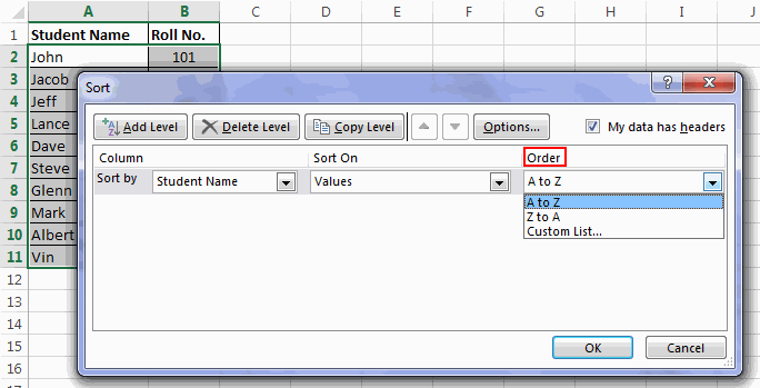
First of all, select the table to be alphabetized.

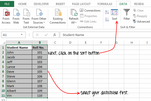
After this click the “Sort” button, on the “Data” tab.

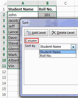
This will open a “Sort” dialog box, in the ‘Column’ dropdown select the column based on which you want to alphabetize your data.

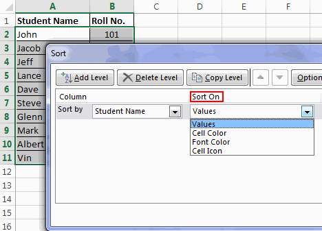
In the ‘Sort On’ dropdown select the ‘values’ option. Using ‘Sort On’ dropdown you can sort your data based on cell colour, font colour or cell icons.

In the ‘Order’ field select “A-Z” for Ascending sort or “Z-A” for descending sort. If your data is without a header row then uncheck the ‘My data has headers’ checkbox, otherwise, leave it checked.

Finally, click on the ‘Ok’ button and your data is sorted.

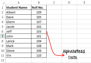
Notice that the names are sorted but the corresponding roll numbers have not changed, so the data is still reliable.

Method 2 – Alphabetizing a column using shortcut keys

If you are someone who uses the keyboard more to perform the same tasks with the mouse, I will share here a list of keyboard shortcuts that will come in handy when arranging columns in Excel.

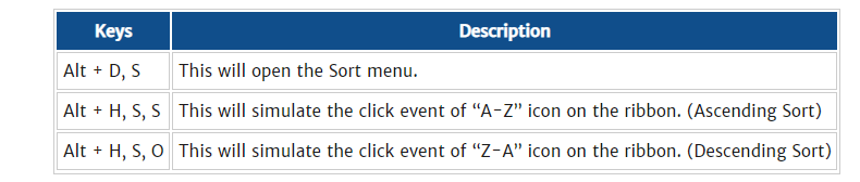
Note Before using these keyboard shortcuts, make sure that you have already selected the data table.

Method 3 – Follow the list using an Excel formula:

In this method, we will use Excel formulas to sort the list alphabetically. The two formulas we use are COUNTIF and VLOOKUP.

Many of you will think, “How do we sort the list using the CountIf function?” The trick behind this is that we can use the COUNTIF function to calculate values based on specific behavior.

For example: Suppose we have a list with some alphabets 'o, l, n, m, p, q' in a range A1:A6. Now if we use a formula as:

=COUNTIF(“A1:A6″,”>o”)

The result can be 3, because only three alphabets (l, m, n) mean “o”. This clearly shows that the COUNTIF function can give us a sort when used correctly.

We will use this concept in our previous example.

First, we’ll create a temporary column called “Subsequent” in our existing table. Next, we use the formula = COUNTIF ($ B $ 2: $ B $ 11, “<=” & B2) for the first student.

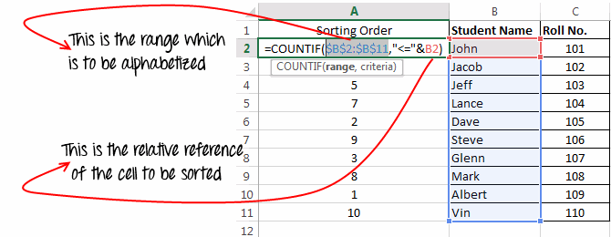
And then we drag and drop this formula to fill it in its entirety.

This formula indicates the order in which the items in the list are arranged. Now we only need to sort the data based on sorting and we will use the VLOOKUP function to do that.

=VLOOKUP(<sort number>,A:B,2,0)

Here, “type number” means numbers in ascending order from 1 to 10. For descending order, the numbers should be from 10-1.

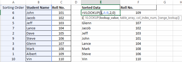
Similarly, for the second and third items, you can use the formula as :=VLOOKUP(2,A:B,2,0)

and=VLOOKUP(3,A:B,2,0)

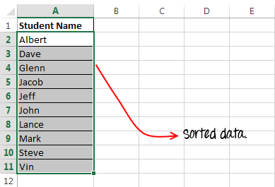
After applying this VlookUp formula the list gets alphabetized.

Tip: Instead of manually entering the 1-10 in the above formula, you can also use the row function to ease your task. Row() gives you the row number of the current cell.

So, with the use of the row function the formula would be:

=VLOOKUP(ROW()-1,A:B,2,0)

So, this was all about how to alphabetize in excel. Do share your thoughts about this topic.

Related Blogs –